CheckM2
Metagenomic BinningCheckM2 is a rapid machine-learning-based tool for assessing the quality of metagenome-assembled genomes (MAGs). It uses gradient-boosted models trained on genomic features to predict completeness and contamination without requiring reference genomes. [1]
How to Obtain Output Model File
Below is a brief workflow the team ran to obtain the output model examples we present on the tools page.
Input
Directory of genome bins in FASTA format (.fa, .fna, .fasta)
Output
TSV file with per-bin quality metrics: completeness, contamination, coding density, GC content, genome size, N50, contig count
conda install -c bioconda checkm2
Docker image: nanozoo/checkm2:latest
Sample 1 21 metagenome-assembled bins from the PRJNA795985 gut microbiome co-assembly assessed with CheckM2 using the Database.
- 1
Download 3 samples from PRJNA795985
for SRR in SRR17531757 SRR17531762 SRR17531772; do fastq-dump --split-files --gzip -X 1000000 --outdir reads/ $SRR; done
1M read pairs per sample from "Diet and Antimicrobial Resistance in Healthy US Adults" (Shrestha et al., mBio 2022).
- 2
Co-assemble with MEGAHIT
megahit -1 reads/SRR17531757_1.fastq.gz,reads/SRR17531762_1.fastq.gz,reads/SRR17531772_1.fastq.gz -2 reads/SRR17531757_2.fastq.gz,reads/SRR17531762_2.fastq.gz,reads/SRR17531772_2.fastq.gz -o assembly --min-contig-len 1500 -t 8
Co-assembly produces 14,934 contigs (≥1,500 bp).
- 3
Map each sample to contigs
for SRR in SRR17531757 SRR17531762 SRR17531772; do minimap2 -ax sr -t 8 assembly/final.contigs.fa reads/${SRR}_1.fastq.gz reads/${SRR}_2.fastq.gz | samtools sort -@ 4 -o bams/${SRR}.sorted.bam && samtools index bams/${SRR}.sorted.bam; doneProduces per-sample BAM alignments required for binning.
- 4
Bin contigs
vamb bin default --outdir vamb_out --fasta assembly/final.contigs.fa --bamdir bams/ -m 1500 --minfasta 200000 -p 8
Produces 21 bin FASTA files (≥200 Kbp).
- 5
Download CheckM2 database
checkm2 database --download --path checkm2_db/
Downloads the DIAMOND database (uniref100.KO.1.dmnd, ~1.74 GB).
- 6
Run CheckM2 on all 21 bins
checkm2 predict --input bins/ --output-directory checkm2_output/ -x fna --threads 8 --database_path checkm2_db/uniref100.KO.1.dmnd
Produces quality_report.tsv with completeness, contamination, coding density, GC content, N50, and genome size for all 21 bins.
quality_report.tsv to IntMetaMaterials Used
Charts Reference
Detailed descriptions for all 13 visualizations generated by CheckM2 in IntMeta.
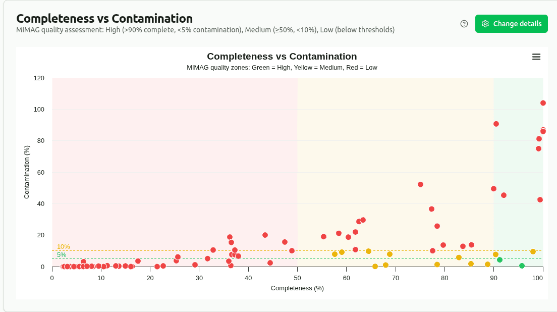
completeness-vs-contamination
Scatter plot of ML-predicted completeness (%) vs contamination (%) for each bin, colored by MIMAG quality tier. Ideal bins sit in the top-left corner. Dashed lines mark MIMAG thresholds: High quality (≥90% complete, <5% contamination) and Medium quality (≥50% complete, <10% contamination).
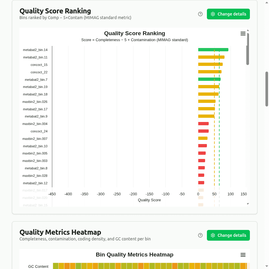
quality-score-ranking
Horizontal bar chart ranking bins by composite quality score = Completeness − 5 × Contamination (the standard MIMAG formula). A bin with 95% completeness and 2% contamination scores 85. Color reflects the MIMAG quality tier (High / Medium / Low).
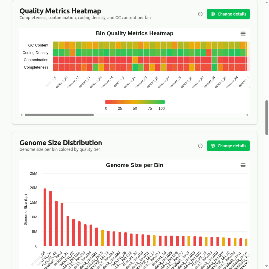
quality-metrics-heatmap
Heatmap of min-max normalized values of Completeness, Contamination, Coding_Density, and GC_Content across all bins. Each metric is scaled 0–1 within its column; darker cells indicate higher relative values. Useful for spotting outlier bins at a glance.
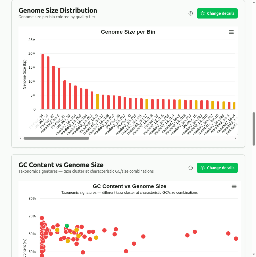
genome-size-distribution
Bar chart of Genome_Size (Mbp) per bin, sorted by size and colored by MIMAG quality tier. Dashed reference lines indicate typical bacterial genome size ranges (most are 1–8 Mbp). Unusually small or large bins may warrant manual inspection.

gc-content-vs-genome-size
Scatter plot of GC_Content (%) vs Genome_Size. Different taxa cluster at characteristic GC/size combinations — e.g., Firmicutes tend toward 30–40% GC while Actinobacteria often exceed 60%. Outlier positions may indicate chimeric bins mixing contigs from unrelated organisms.
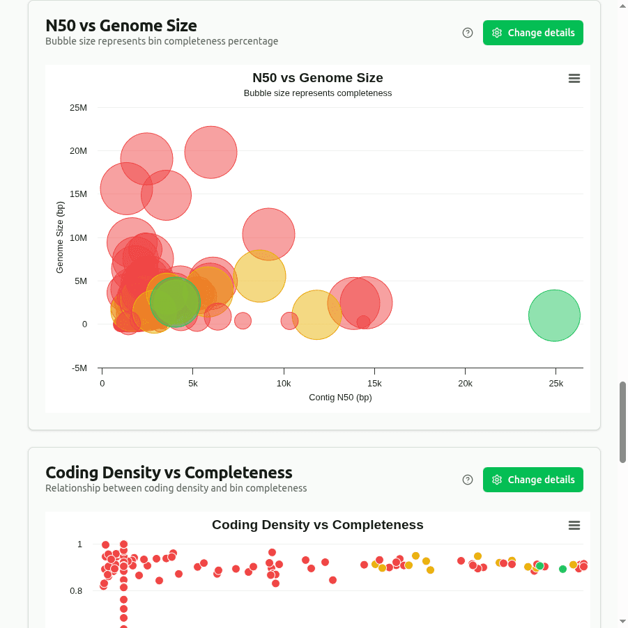
n50-vs-genome-size
Bubble plot where X = Genome_Size, Y = Contig_N50 (half the assembly length is in contigs ≥ this size), and bubble diameter = Completeness (%). Top-right, large bubbles represent well-assembled, complete genomes.
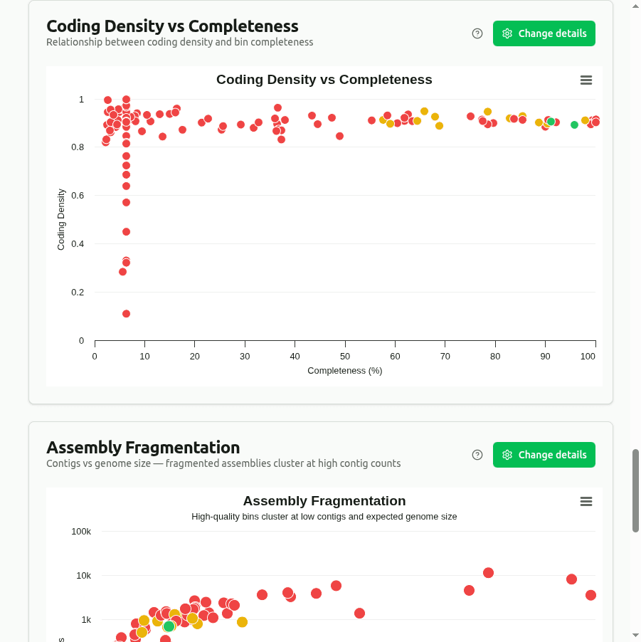
coding-density-vs-completeness
Scatter plot of Coding_Density (fraction of bases in coding sequences) vs Completeness, colored by quality tier. Most prokaryotic genomes have coding density between 85–95%. Low coding density combined with high completeness may signal contamination with non-coding DNA.

assembly-fragmentation
Scatter plot of Total_Contigs (contig count) vs Genome_Size. Highly fragmented assemblies appear upper-left (many contigs, small genome). Well-assembled genomes cluster lower-right (few contigs, large genome). Fragmentation affects downstream analyses like gene prediction.

comp-quality-tiers
Grouped bar chart comparing the distribution of MIMAG quality tiers (High / Medium / Low) across samples. Each group shows one bar per sample, enabling quick assessment of which sample produced higher-quality bins overall.

comp-genome-size
Box plot or grouped bar chart comparing the genome size distribution of bins across samples. Reveals whether certain samples yield systematically larger or smaller MAGs, which may reflect community composition differences.
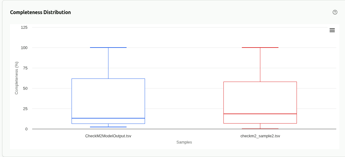
comp-completeness
Box plot comparing the distribution of ML-predicted completeness (%) across samples. Higher medians and tighter interquartile ranges indicate more consistently complete bins in that sample.
comp-contamination
Box plot comparing contamination (%) distribution across samples. Lower values are better — samples with elevated contamination may need stricter binning parameters or additional refinement.
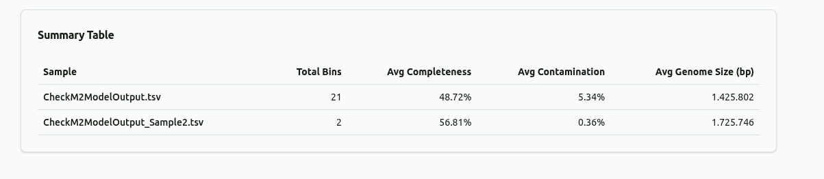
comp-summary-table
Aggregate summary table showing key metrics per sample: total number of bins, mean completeness, mean contamination, mean genome size, and number of high-quality bins. Provides a quick numerical overview for cross-sample comparison.